Catenary Curve

Aside: The catenary equations are related to grade school geometry in the same way that dinner from a Michelin restaurant is related to a can of beans. They can both be consumed, but one is a bit more involved.

We have looked at some standard geometric curves, such as circles, ellipses, parabolas and hyperbolas. Now we want to look at one that occurs whenever a cable is suspended from both ends and allowed to hang down under the force of gravity. Some examples of the catenary curve are an electric line between two poles, an anchor line from the seabed to a boat, or a chain between two posts along a walkway. The question is how to describe the locus of points that position the cable. There are many nuances to the question and we will not try to address them all, but we need to be careful that with alternative physical models, all of the forces which might affect the curve are considered. Often they are subtle.

The equation that describes a catenary curve is derived by adhering to some laws of physics. Often it is the main topic for any discussion about these curves. However, it is technical, tedious and not overly useful for problem solving. Consequently, we will put it into a subsection and you may look at it if you want. Otherwise, we are going to just define a catenary equation and focus on solving a few practical examples.

The catenary curve that we would graph has the equation $$f(x)=a\cdot cosh\left(\frac{x}{a}\right).\tag{1} \label{1}$$ There is nothing simple about this equation. It is a function of $x$ which is still defined in the usual sense of a number line and $f(x)$ is still the orthogonal coordinate value, but we have a hyperbolic cosine and an undefined variable, $a$. As we have described the application of a suspended cable, $x$ is taken to the be a linear axis distance from the lowest sag point of the cable to one of the suspension points. In working with the equation, we will nearly always put the $y$-axis directly through the lowest sag point of the cable. As for the $x$-axis, as the equation is described in $\eqref{1}$ it is $a$ units below that lowest sag point. In this analysis, we will only be considering cables with attachment to eithrer side of a sag point.

Frequently, we will see example problems that ask about the length of cable needed to go between two suspension points and sag a defined amount. While we can (and will) show such examples, they are largely unrealistic. Why? Cable materials stretch. They stretch and contract based on temperature, wind strength, icing, weight of fallen trees, and other unknowns. Usually, the criteria are 1) the cable doesn't break under any atmospheric condition, 2) the cable is kept a minimum distance from the ground under extreme conditions, 3) the cable performs its intended function while minimizing lifetime cost. We will not ignore the cost part of the problem, but we will also not calculate it and instead just specify what cable to use. The more important analyis, rather than length of cable, is what tension will be on the cable at each suspension point because that will determine what cables can be used. They must not break. Sometimes the problems get elaborate. For example, we might see a specification for an ice load equivalent to 3/4 inch (19mm) around a cable that is nominally 0.99 inches (25.15mm). Under these condition we would want to compute the tension at each end of the cable. If it were stretched 0.5 miles from the top of a hill, across a lake, and to a lower attachment point on the other side, how much tension would be on each end? After a suitable margin of error is added, what rated breaking strength would the cable need to have?

Derivation - shorter

Aside: This derivation omits most of the algebra as well as not showing how any of the integrals or derivatives are found.

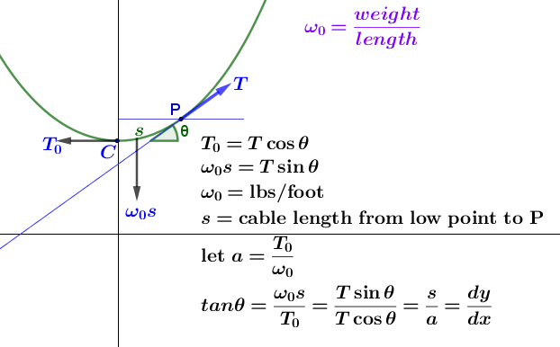
We deal with the cable as the segment from the low point up to some point on the cable named $P.$ We want to balance the horizontal tension, $T_{0},$ the vector tension, $T,$ and the vertical gravitational pull on the cable, $\omega_{0}s,$ where $\omega_{0}$ is the cable weight/length and $s$ is the segment of cable from the low point to $P.$

The tension is tangent to the curve at all points. At point $C,$ the tension is balanced between the left and right halves. We develop the equations for the right half. $T_{0}$ is clearly not equal to zero as it must pull the right section to the left. The tension, $T,$ must be $(T\cos\theta,T\sin\theta)$ when expressed as its horizontal and vertical components. $\theta$ is the usual angle between the tangent line and the horizontal axis. The vertical component is the weight of the chain segment, $\omega_{0}s.$ So we get two equations. $$\text{horizontal: }T_{0}=T\cos\theta$$ $$\text{vertical: }\omega_{0}s=T\sin\theta$$ As they are written, these equations are not very useful. We can know $\omega_{0}.$ It is the cable weight per unit length. We might know $s$ but it may also be something we want to solve for. We probably do not know $T$ or $T_{0}$ and $\theta$ is a moving target. So, express the tangent as (see figure 1) $$\tan\theta=\frac{\omega_{0}s}{T_{0}}=\frac{dy}{dx}=y^{\prime}. \tag{2} \label{2}$$ In $\eqref{2}$ we have a single differential equation. The variables $x$ and $y$ refer to the coordinates of any point on the curve. Also, both $\omega_{0}$ and $T_{0}$ are constants, although $T_{0}$ is not a known constant. What is typically done is to define a new constant, $a=T_{0}/\omega_{0}$ and substitute that into $\eqref{2}$ giving $$y'=\frac{s}{a}.$$ Next we do something really clever and note from prior experience that $s$ is just an arc length and we know arc length to be $$s=\int\sqrt{1+\left(\frac{dy}{dx}\right)^{2}}dx$$ and since $dy/dx=s/a,$ $$s=\int\sqrt{1+\left(\frac{s}{a}\right)^{2}}dx.$$ Next we can take the derivative of both sides, $$\frac{ds}{dx}=\sqrt{1+\left(\frac{s}{a}\right)^{2}}=\frac{\sqrt{a^{2}+s^{2}}}{a}$$ which rearranges to $$\frac{1}{\sqrt{a^{2}+s^{2}}}ds=\frac{1}{a}dx.$$ Now integrate both sides, $$\int\frac{1}{\sqrt{a^{2}+s^{2}}}ds=\frac{1}{a}\int dx$$ This next step is a leap (see Catenary 'more detail'), $$\sinh^{-1}\left(\frac{s}{a}\right)=\frac{x}{a}$$ and $$\frac{s}{a}=\sinh\left(\frac{x}{a}\right)+const.$$ Since $s/a=dy/dx,$ and we know that at $x=0,$ $dy/dx=0$ because that is the low point of the curve, then the constant is zero. Also, and again because $s/a=dy/dx,$ we get $$y'=\sinh\left(\frac{x}{a}\right)$$ which integrates to $$y=a\cosh\left(\frac{x}{a}\right)+const.$$ We evaluate the constant from $x=0,$ then $y=a.$ In order to make our latest constant be zero, we have to shift the $x$-axis such that at $x=0$ then $y=a.$ Finally, the two working equations are $$\frac{s}{a}=\sinh\left(\frac{x}{a}\right)\quad\text{and}\quad f(x)=a\cosh\left(\frac{x}{a}\right).$$